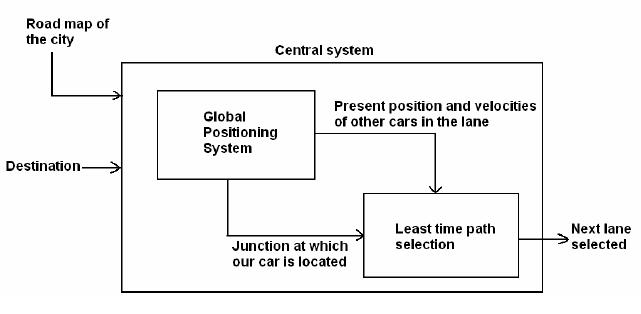
Central System

The Global Positioning System (GPS) is formed from an array of 24 satellites orbiting 24,000 kilometers (14,900 miles) above the Earth that orbit the earth twice a day. The basis of GPS is triangulation. Mathematically we need only three distances from satellites to get the coordinates of the GPS receiver (But here practically we use four for technical reasons). Distances can be calculated by time taken for radio waves from satellite to GPS receiver. GPS technology uses a clever way to calculate the time taken for travel. Each satellite generates its gpseudo random codeh (just a complex digital code which consists of on/off pulses) same code is generated at GPS receiver, so what reaches the receiver is delayed version of the signal. Radio waves take finite time to reach the GPS receiver until it syncs up with the satellite's code (correlation of the received code with receivers code reaches maximum). The amount we have to shift back the receiver's version is equal to the travel time of the satellite's version. Inverted Differential GPS (DGPS) is a cheap way for improving navigation accuracies in local area which is what we require in our application. Each car would be equipped with standard receiver and a transmitter to transmit back to tracking office their central system which ties all satellite measurements into a solid local reference.

We give as inputs the origin and destination of our journey to the central system. The central system has the map of city and continuously monitors the positions and velocities of all the cars in the lanes through GPS. We want to reach our destination in shortest time possible. The central command system optimizes travel path to travel in shortest time possible. It basically has to solve "shortest-paths problem" to be more precise "single-pair shortest-path problem" at every junction when a decision is required.

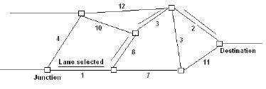
Description of single-pair shortest-path problem
In this problem, we are given a weighted, directed graph G = (V, E), with weight function w: E¨(to) R mapping edges to real valued weights and two vertices u, v belonging to V. The weight of the path p is sum of weights of its constituent edges

w(p) = summation ofw(pi, pi-1) p0 = u pk = v
We have to find the shortest path from u to v where shortest path is defined as path with weight of the path being less than or equal to minimum of the weight of the all paths connecting the u and v.
No algorithm for the single-pair shortest-path problem is known to run faster the single-source algorithms (to find the shortest path from a single source to all vertices). We solve single source shortest path using Dijkstrafs algorithm (here the weights is time taken to travel the lane is always non negative)

Application to our problem with
V as the junctions of the city
E as the lane joining the junctions
w as the estimated time taken to travel the lane.

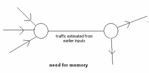
System properties of w
It takes as inputs, the positions and velocities of the all cars and the length of the road. It is the most important calculation for the system is dependent on various factors. It is not entirely dependent on the present input because when the time the car travels in the lane the traffic would have changed, but it would be dependent on the traffic in lanes connecting to the junction at some previous instant and turn ratios (we have to estimate the probability from data collected over period of time). So this system needs to have memory because of the fact that when the decision for shortest path is also being taken on basis of predicted from traffic at earlier instants and collected turn ratios over time.



We consider other dependencies to model the real life situation like there is a road block due to some accident (in this case we have to consider the time taken to be infinite to cross the lane as the person would not want to wait for long time). All thought the input is bounded, output for weight function is considered to be infinite for calculation purpose. Suppose the road is under heavy traffic, then it would take us lot of time to reach our destination. In this case we have finite number of cars on the road (saturation) and all have very low speeds due to congestion, thus the input can be said to be bounded. But till it will increase the weight function infinitely, thus the output is unbounded.

Calculations cant be made using linearity principle. This can be proved by counter example - suppose traffic doubles, the time taken to cross the lane does more than the double of the initial value, as the number of cars is doubled, the speed of each car decreases and thus the final weight function is more than the double of the initial value.
Weight function for present traffic can be copied from the similar past traffic (here presents and past refers to time period day). This is very helpful as in weekdays traffic is almost similar, we improve the present estimation because mostly past weight functions would be repeated. Weight of the path as defined above adds up the total time taken to travel between two junctions By solving this problem we get the path which takes the shortest time between the two junctions and thereby the next lane to be taken from the junction.

Our car starts from origin it receives from the central system the lane to be taken at the junction depending on the weight function estimation which is calculated from continuous GPS monitoring. It uses the internal control system to move through until it reaches the next junction. On reaching the next junction it again receives the lane to be taken from the central system depending on the then calculated weight function.

position = origin
while (position is not equal to destination)
ASK_LANE(position)
ASK_LANE(position)
FIRST_EDGE(SHORTEST_PATH(position, destination))
SHORTEST_PATH is calculated using the weight function derived as in the discussion above.
FIRST_EDGE is the starting edge in the shortest path thus calculated.